Chapter 3 - Classification

Binary Classifier - a classifier capable of distinguishing between 2 classes

Stochastic Gradient Descent (SGD) classifier:
capable of handling very large datasets efficiently, because SGD deals with training instances independently, one at a time (which also makes SGD well suited for online learning), as we will see later.

Note on SGD: The SGDClassifier relies on randomness during training (hence the name “stochastic”). If you want reproducible results, you should set the random_state parameter.

Confusion matrix

Count the number of times instances of class A are classified as class B. For example, to know the number of times the classifier confused images of 5s with 3s, you would look in the fifth row and third column of the confusion matrix

Each row in a confusion represents an actual class
Each column in a confusion matrix represents a predicted class

For instance:


from sklearn.metrics import confusion_matrix
confusion_matrix(y_train_5,y_train_pred)

Output:
       # N         #P
 array([[53057,  1522], #N
     [ 1325,  4096]])   #P

The first row of this matrix considers non-5 images (the negative class): 53,057 of them were correctly classified as non-5s (they are called true negatives), while the remaining 1,522 were wrongly classified as 5s (false positives).
The second row considers the images of 5s (the positive class): 1,325 were wrongly classified as non-5s (false negatives), while the remaining 4,096 were correctly classified as 5s (true positives).
A perfect classifier would have only true positives and true negatives, so its confusion matrix would have nonzero values only on its main diagonal

The confusion matrix gives you a lot of information, but sometimes you may prefer a more concise metric. An interesting one to look at is the accuracy of the positive predictions; this is called the precision of the classifier
precision is typically used along with another metric named recall, also called sensitivity or the true positive rate (TPR): this is the ratio of positive instances that are correctly detected by the classifier
It is often convenient to combine precision and recall into a single metric called the F1 score, in particular if you need a simple way to compare two classifiers. The F1 score is the harmonic mean of precision and recall (Equation 3-3). Whereas the regular mean treats all values equally, the harmonic mean gives much more weight to low values. As a result, the classifier will only get a high F1 score if both recall and precision are high.

The F1 score favors classifiers that have similar precision and recall. This is not always what you want: in some contexts you mostly care about precision, and in other contexts you really care about recall.

For example, if you trained a classifier to detect videos that are safe for kids, you would probably prefer a classifier that rejects many good videos (low recall) but keeps only safe ones (high precision), rather than a classifier that has a much higher recall but lets a few really bad videos show up in your product (in such cases, you may even want to add a human pipeline to check the classifier’s video selection).

On the other hand, suppose you train a classifier to detect shoplifters in surveillance images: it is probably fine if your classifier has only 30% precision as long as it has 99% recall (sure, the security guards will get a few false alerts, but almost all shoplifters will get caught)

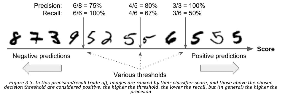
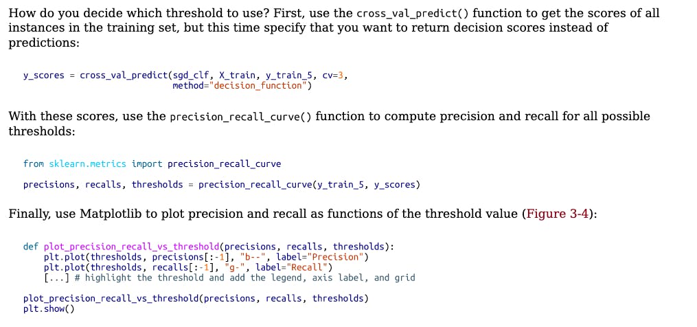
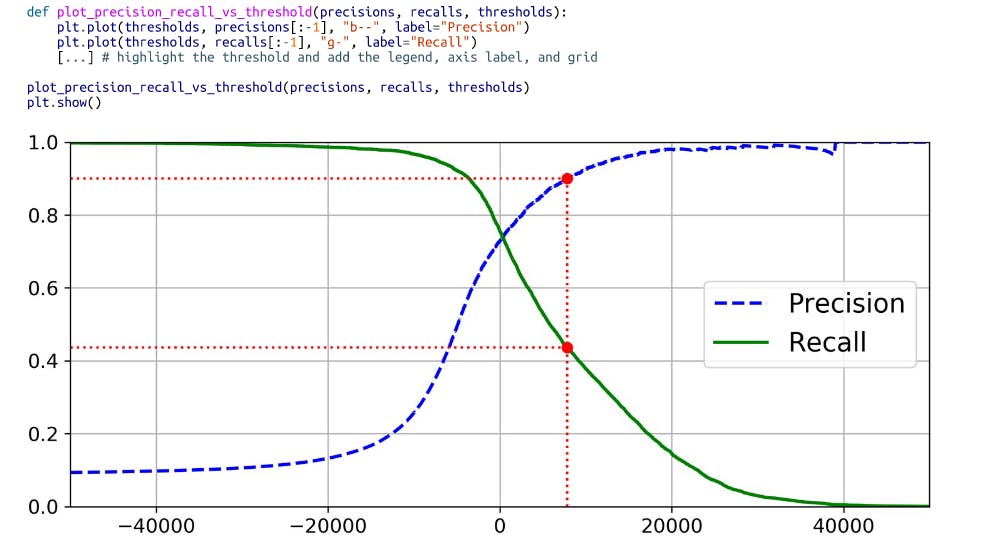
Precision/Recall trade-off

let’s look at how the makes its classification decisions. For each instance, it computes a score based on a decision function. If that score is greater than a threshold, it assigns the instance to the positive class; otherwise it assigns it to the negative class

Suppose the decision threshold is positioned at the central arrow (between the two 5s): you will find 4 true positives(actual 5s) on the right of that threshold, and 1 false positive (actually a 6). Therefore, with that threshold,the precision is 80% (4 out of 5). But out of 6 actual 5s, the classifier only detects 4, so the recall is 67% (4out of 6). If you raise the threshold (move it to the arrow on the right), the false positive (the 6) becomes a true negative, thereby increasing the precision (up to 100% in this case), but one true positive becomes a false negative, decreasing recall down to 50%. Conversely, lowering the threshold increases recall and reduces precision.

The ROC Curve

Similar to precision/recall curve, but instead of plotting precision vs recall, it plots the true positive rate vs false positive rate.
The FPR is the ratio of negative instances that are incorrectly classified as positive. It is equal to 1 – the true negative rate (TNR), which is the ratio of negative instances that are correctly classified as negative. The TNR is also called specificity. Hence, the ROC curve plots sensitivity (recall) versus 1 – specificity.

Multiclass Classification

Some algorithms (such as SGD classifiers, Random Forest classifiers, and naive Bayes classifiers) are capable of handling multiple classes natively. Others (such as Logistic Regression or Support Vector Machine classifiers) are strictly binary classifiers
One way to create a system that can classify the digit images into 10 classes (from 0 to 9) is to train 10binary classifiers, one for each digit (a 0-detector, a 1-detector, a 2-detector, and so on). Then when you want to classify an image, you get the decision score from each classifier for that image and you select the class whose classifier outputs the highest score. This is called the one-versus-the-rest (OvR) strategy (also called one-versus-all)
Another strategy is to train a binary classifier for every pair of digits: one to distinguish 0s and 1s, another to distinguish 0s and 2s, another for 1s and 2s, and so on. This is called the one-versus-one (OvO) strategy.If there are N classes, you need to train N × (N – 1) / 2 classifiers.
For the MNIST problem, this means training 45 binary classifiers! When you want to classify an image, you have to run the image through all 45classifiers and see which class wins the most duels. The main advantage of OvO is that each classifier only needs to be trained on the part of the training set for the two classes that it must distinguish.

Error Analysis

-First, look at the confusion matrix

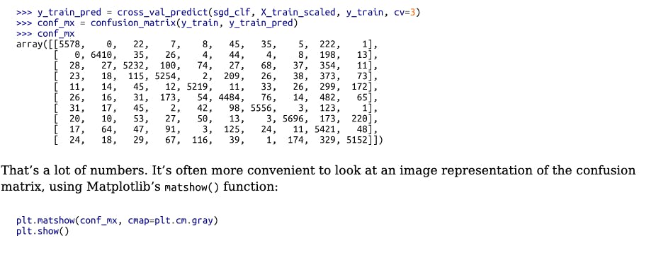
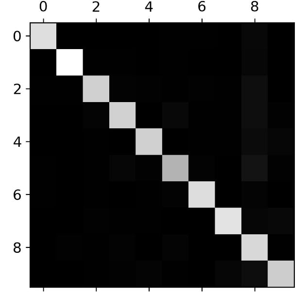
This confusion matrix looks pretty good, since most images are on the main diagonal, which means thatthey were classified correctly. The 5s look slightly darker than the other digits, which could mean that thereare fewer images of 5s in the dataset or that the classifier does not perform as well on 5s as on other digits.
In fact, you can verify that both are the case.Let’s focus the plot on the errors. First, you need to divide each value in the confusion matrix by the number of images in the corresponding class so that you can compare error rates instead of absolute numbers of errors (which would make abundant classes look unfairly bad):


mtx = confusion_matrix(y_train,sgd_clf.predict(X_train))
row_mtx = mtx.sum(axis=1,keepdims=True)
norm_conf_mtx = mtx / row_mtx

np.fill_diagonal(norm_conf_mtx,0)
sns.heatmap(norm_conf_mtx,cmap='plasma')

The Machine Learning Engineer Club